> pixi add jupyterlab pandas matplotlib seaborn --pypiPython
What is Python?
Python is a high-level, general-purpose programming language that is widely used in data science, machine learning, and web development. It has a large standard library and a vibrant community that provides a wide range of libraries and tools for various applications. As such, Python provides a general-purpose ecosystem that can be used for a wide range of applications.
How to install Python?
There are many ways to install Python. We recommend using Python in a virtual environment to avoid conflicts with other Python installations on your system.
We recommend using pixi as a a simple way to create and manage Python virtual environments.
You can manage the python packages that are installed in the virtual environment using a pyproject.toml file. See the pyproject.toml example in this repository for an example of how to manage Python packages. To add package dependencies to the virtual environment, using pixi, you can run:
First, install pixi using winget (Windows) or brew (MacOS/Linux):
| Platform | Commands |
|---|---|
| Windows | winget install prefix-dev.pixi |
| MacOS | brew install pixi |
| Linux | brew install pixi |
Add libraries to the virtual environment using pixi add ...:
Coding Conventions
We highly recommend working with a virtual environment to manage Python dependencies. The pyproject.toml is the preferred way to keep track of python dependencies as well as project-specific python conventions.
We recommend using Ruff to enforce linting and formatting rules. In most cases you can use the default linting and formatting rules provided by ruff. However, you can customize the rules by modifying the [tool.ruff] section of the pyproject.toml file in the root of your project. for more about the configuration options, see the Ruff documentation.
If you are working in a virtual environment created in this repository, you automatically have access toRuff via just lint-py and just fmt-python commands to lint and format your code.
For more inspiration, see the GitLab Data Team’s Python Guide and Google’s Python Style Guide.
Example Usage
Let’s load an example World Bank data via Gapminder using the causaldata package.
import pandas as pd
import matplotlib.pyplot as plt
import seaborn as sns
import statsmodels.formula.api as sm
from causaldata import gapminder
Load the Gapminder data as a pandas DataFrame:
df = gapminder.load_pandas().dataWe can check the dimensions of the DataFrame using df.info():
df.info()<class 'pandas.core.frame.DataFrame'>
RangeIndex: 1704 entries, 0 to 1703
Data columns (total 6 columns):
# Column Non-Null Count Dtype
--- ------ -------------- -----
0 country 1704 non-null object
1 continent 1704 non-null object
2 year 1704 non-null int64
3 lifeExp 1704 non-null float64
4 pop 1704 non-null int64
5 gdpPercap 1704 non-null float64
dtypes: float64(2), int64(2), object(2)
memory usage: 80.0+ KBLet’s take a look at the first few rows of the DataFrame using df.head():
df.head()| country | continent | year | lifeExp | pop | gdpPercap | |
|---|---|---|---|---|---|---|
| 0 | Afghanistan | Asia | 1952 | 28.801 | 8425333 | 779.445314 |
| 1 | Afghanistan | Asia | 1957 | 30.332 | 9240934 | 820.853030 |
| 2 | Afghanistan | Asia | 1962 | 31.997 | 10267083 | 853.100710 |
| 3 | Afghanistan | Asia | 1967 | 34.020 | 11537966 | 836.197138 |
| 4 | Afghanistan | Asia | 1972 | 36.088 | 13079460 | 739.981106 |
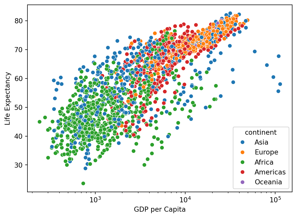
Take a look at the relationship between GDP per Capita and Life Expectancy:
sns.scatterplot(x="gdpPercap", y="lifeExp", hue="continent", data=df).set(
    xscale="log", ylabel="Life Expectancy", xlabel="GDP per Capita"
)
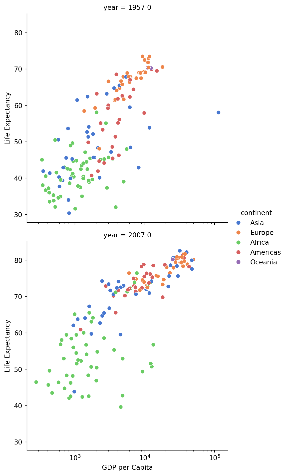
Separate the data by year, focusing on 1957 and 2007:
sns.relplot(
    data=df.where(df["year"].isin([1957, 2007])),
    x="gdpPercap",
    y="lifeExp",
    col="year",
    hue="continent",
    col_wrap=1,
    kind="scatter",
    palette="muted",
).set(xscale="log", ylabel="Life Expectancy", xlabel="GDP per Capita")